How to use the PivotTable in the MS-Excel during your professional and business life.
How to use the PivotTable in the MS-Excel during your professional and business life.
Use the following step to use the PivotTable in MS-Excel.
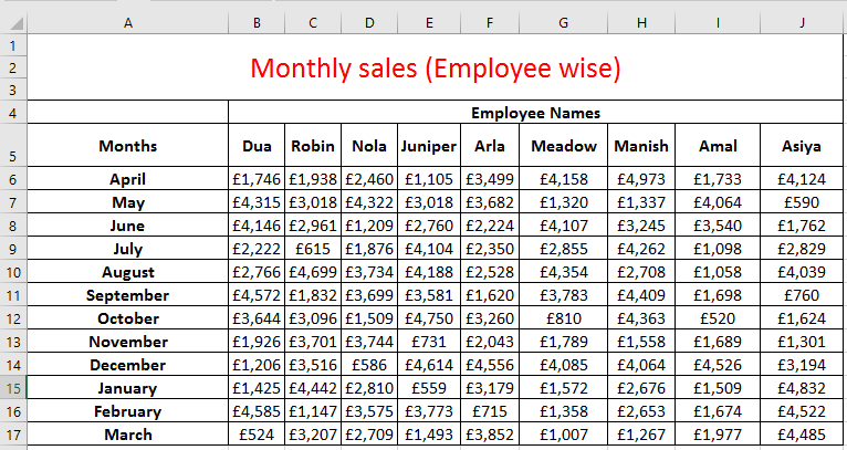
1. Arrange your data properly in the MS-Excel worksheet(like as below) and select the whole database or table.
3. Then below dialog box will appear in the
MS-Excel sheet and select the new worksheet or select the cells where you want
to place the Pivot table (in professional work you should use the new
worksheet) and then click on the OK button.
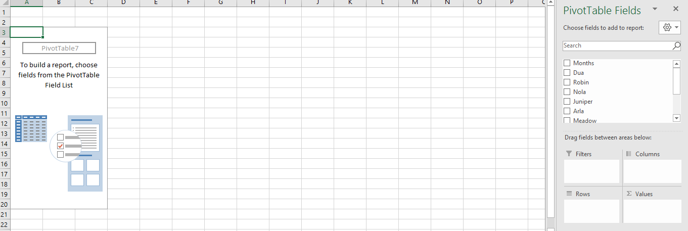
4. Now PivotTable option will appear in the MS-Excel worksheet, and you find the screen like this.
5. Now drop the months in rows box and other
valuable data into the value box.
6. Now your PivotTable will appear as below in the MS-Excel sheet.
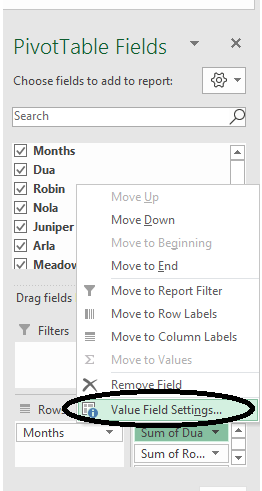
8. After selecting the Value Field Settings and select the information you want like count, minimum and maximum, etc., now select the average option and press ok in the MS-Excel.
9. Now you got the average sale of Dua at the bottom of the table in the MS-Excel worksheet.
10. Same you can also try the same with others.
In upcoming days I also share the other functions that use
in the PivotTable like charts, sorting, and many others.
If you have any queries or questions related to PivotTable
or any other MS-Excel tool and even if you want the online practical training
or special online lecture one to one then contact me on my below details.
Manish Kumar,
Student at Ulster University,
You also follow me and give feedback on my Facebook page knowledgeforexcel,
Instagram page knowledge4excel, and twitter knowledge4excel.


Comments
Post a Comment